Timeseries AIT Tutorial

The goal of this notebook is to use the trained AIT model to calculate expected energy levels based on field data. First we will load in and clean the data and after the expected energy is calculated, we will create comparitive visualizations.

import numpy as np
import pandas as pd
import matplotlib.pyplot as plt
import os

from pvops.timeseries import preprocess
# from pvops.timeseries.models import linear, iec, AIT
from pvops.text2time import utils as t2t_utils, preprocess as t2t_preprocess

Load in data

example_OMpath = os.path.join('example_data', 'example_om_data2.csv')
example_prodpath = os.path.join('example_data', 'example_prod_with_covariates.csv')
example_metapath = os.path.join('example_data', 'example_metadata2.csv')

prod_data = pd.read_csv(example_prodpath, on_bad_lines='skip', engine='python')

prod_data.head(5)

	date	randid	generated_kW	expected_kW	irrad_poa_Wm2	temp_amb_C	wind_speed_ms	temp_mod_C
0	2018-04-01 07:00:00	R15	0.475	0.527845	0.02775	16.570	4.2065	14.1270
1	2018-04-01 08:00:00	R15	1332.547	1685.979445	87.91450	16.998	4.1065	15.8610
2	2018-04-01 09:00:00	R15	6616.573	7343.981135	367.90350	20.168	4.5095	24.5745
3	2018-04-01 10:00:00	R15	8847.800	10429.876422	508.28700	21.987	4.9785	30.7740
4	2018-04-01 11:00:00	R15	11607.389	12981.228814	618.79450	23.417	4.6410	35.8695

metadata = pd.DataFrame()
metadata['randid'] = ['R15', 'R10']
metadata['dcsize'] = [25000, 25000]
metadata.head()

	randid	dcsize
0	R15	25000
1	R10	25000

Column dictionaries

Create production and metadata column dictionary with format {pvops variable: user-specific column names}. This establishes a connection between the user’s data columns and the pvops library.

prod_col_dict = {'siteid': 'randid',
                 'timestamp': 'date',
                 'powerprod': 'generated_kW',
                 'energyprod': 'generated_kW',
                 'irradiance':'irrad_poa_Wm2',
                 'temperature':'temp_amb_C', # Optional parameter, used by one of the modeling structures
                 'baseline': 'AIT', #user's name choice for new column (baseline expected energy defined by user or calculated based on IEC)
                 'dcsize': 'dcsize', #user's name choice for new column (System DC-size, extracted from meta-data)
                 'compared': 'Compared',#user's name choice for new column
                 'energy_pstep': 'Energy_pstep', #user's name choice for new column
                 'capacity_normalized_power': 'capacity_normalized_power', #user's name choice for new column
}

metad_col_dict = {'siteid': 'randid',
                  'dcsize': 'dcsize'}

Data Formatting

Use the prod_date_convert function to convert date information to python datetime objects and use prod_nadate_process to handle data entries with no date information - here we use pnadrop=True to drop such entries.

prod_data_converted = t2t_preprocess.prod_date_convert(prod_data, prod_col_dict)
prod_data_datena_d, _ = t2t_preprocess.prod_nadate_process(prod_data_converted, prod_col_dict, pnadrop=True)

Assign production data index to timestamp data, using column dictionary to translate to user columns.

prod_data_datena_d.index = prod_data_datena_d[prod_col_dict['timestamp']]

min(prod_data_datena_d.index), max(prod_data_datena_d.index)

(Timestamp('2018-04-01 07:00:00'), Timestamp('2019-03-31 18:00:00'))

Data Preprocessing

Preprocess data with prod_inverter_clipping_filter using the threshold model. This adds a mask column to the dataframe where True indicates a row to be removed by the filter.

masked_prod_data = preprocess.prod_inverter_clipping_filter(prod_data_datena_d, prod_col_dict, metadata, metad_col_dict, 'threshold', freq=60)

filtered_prod_data = masked_prod_data[masked_prod_data['mask'] == False].copy()
del filtered_prod_data['mask']

print(f"Detected and removed {sum(masked_prod_data['mask'])} rows with inverter clipping.")

Detected and removed 24 rows with inverter clipping.

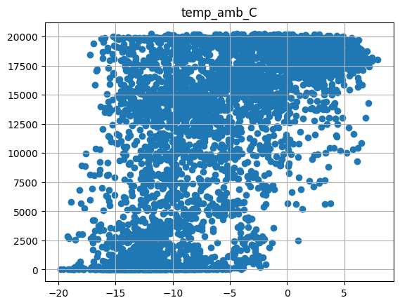
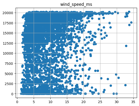
Visualize the power signal versus covariates (irradiance, ambient temp, wind speed) for one site

temp = filtered_prod_data[filtered_prod_data['randid'] == 'R10']
for xcol in ['irrad_poa_Wm2', 'temp_amb_C', 'wind_speed_ms']:
    plt.scatter(temp[xcol], temp[prod_col_dict['powerprod']])
    plt.title(xcol)
    plt.grid()
    plt.show()

Add a dcsize column to production data and populate using site metadata.

filtered_prod_data.head(5)
# metad.to_dict()

	date	randid	generated_kW	expected_kW	irrad_poa_Wm2	temp_amb_C	wind_speed_ms	temp_mod_C
date
2018-04-01 07:00:00	2018-04-01 07:00:00	R15	0.475	0.527845	0.02775	16.570	4.2065	14.1270
2018-04-01 08:00:00	2018-04-01 08:00:00	R15	1332.547	1685.979445	87.91450	16.998	4.1065	15.8610
2018-04-01 09:00:00	2018-04-01 09:00:00	R15	6616.573	7343.981135	367.90350	20.168	4.5095	24.5745
2018-04-01 10:00:00	2018-04-01 10:00:00	R15	8847.800	10429.876422	508.28700	21.987	4.9785	30.7740
2018-04-01 11:00:00	2018-04-01 11:00:00	R15	11607.389	12981.228814	618.79450	23.417	4.6410	35.8695

filtered_prod_data['dcsize'] = 0
# loop through all sites
for site in filtered_prod_data[prod_col_dict['siteid']].unique():
    # find rows corresponding to site
    site_mask = filtered_prod_data[prod_col_dict['siteid']] == site
    # fill out 'dcsize' column for these rows with the appropriate capacity
    site_metadata = metadata[metadata[prod_col_dict['siteid']] == site]
    filtered_prod_data.loc[site_mask, 'dcsize'] = site_metadata['dcsize'].item()

Visualize energy production for a specific site

filtered_prod_data.loc[filtered_prod_data['randid'] == 'R15',prod_col_dict['energyprod']].plot()

<Axes: xlabel='date'>

Drop rows where important columns are na

model_prod_data = filtered_prod_data.dropna(subset=['irrad_poa_Wm2', 'temp_amb_C', 'wind_speed_ms', 'dcsize', prod_col_dict['energyprod']])
model_prod_data.head(5)

	date	randid	generated_kW	expected_kW	irrad_poa_Wm2	temp_amb_C	wind_speed_ms	temp_mod_C	dcsize
date
2018-04-01 07:00:00	2018-04-01 07:00:00	R15	0.475	0.527845	0.02775	16.570	4.2065	14.1270	25000
2018-04-01 08:00:00	2018-04-01 08:00:00	R15	1332.547	1685.979445	87.91450	16.998	4.1065	15.8610	25000
2018-04-01 09:00:00	2018-04-01 09:00:00	R15	6616.573	7343.981135	367.90350	20.168	4.5095	24.5745	25000
2018-04-01 10:00:00	2018-04-01 10:00:00	R15	8847.800	10429.876422	508.28700	21.987	4.9785	30.7740	25000
2018-04-01 11:00:00	2018-04-01 11:00:00	R15	11607.389	12981.228814	618.79450	23.417	4.6410	35.8695	25000

Dynamic linear modeling

Here we use the AIT model to calculate expected energy based on field data. This is appended to model_prod_data as a new column named ‘AIT’.

model_prod_data = AIT.AIT_calc(model_prod_data, prod_col_dict)

The fit has an R-squared of 0.9120709703427121 and a log RMSE of 7.61637773052697

Visualize results

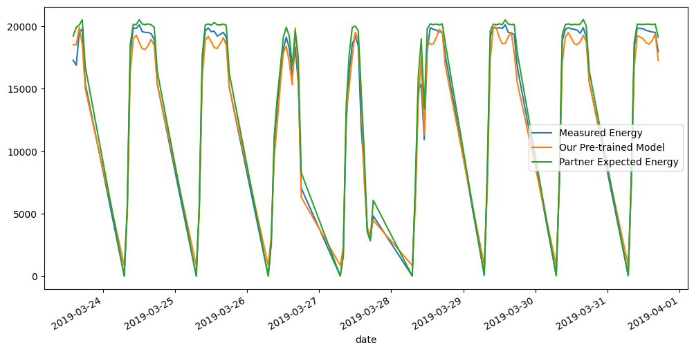
We visualize the measured hourly energy, our pre-trained model’s expected energy, and the results of a partner-produced expected energy over various time-scales.

# defining a plotting utility function
def plot(data, randid, from_idx=0, to_idx=1000):
    data.copy()
    # Just making the visualization labels better here.. for this example's data specifically.
    data.rename(columns={'generated_kW': 'Measured Energy',
                         'AIT': 'Our Pre-trained Model',
                         'expected_kW': 'Partner Expected Energy'}, inplace=True)
    data[data['randid']==randid][['Measured Energy', 'Our Pre-trained Model', 'Partner Expected Energy']].iloc[from_idx:to_idx].plot(figsize=(12,6))

plot(model_prod_data, "R15", from_idx=0, to_idx=100)
plot(model_prod_data, "R15", from_idx=-100, to_idx=-1)

plot(model_prod_data, "R10", from_idx=0, to_idx=100)
plot(model_prod_data, "R10", from_idx=-100, to_idx=-1)