Timeseries Survival Analysis Tutorial
This notebook aims to demonstrate how to perform survival analysis in the context of PV assets, using the methodology from https://ieeexplore.ieee.org/document/9272625/. As outlined in that paper, survival analysis is concerned with estimating the failure rate over the lifetime of a system, given discrete observed failure events.
Gunda et al. used two methods: Kaplan-Meier estimation and fitting a Weibull distribution. We will do both here.
[1]:
import pandas as pd
import matplotlib.pyplot as plt
from pvops import timeseries
WARNING:tensorflow:From c:\Users\agmoore\AppData\Local\anaconda3\envs\pvops\Lib\site-packages\keras\src\backend\common\global_state.py:82: The name tf.reset_default_graph is deprecated. Please use tf.compat.v1.reset_default_graph instead.
Loading and preprocessing data
Reading in data
We read in the data below, where each column reflects data from an O&M (operation and maintenance) ticket. Note the following column descriptions:
randidis an integer identifying the PV siteCODidentifies the commissioning date of the siteEventStartis the recorded time of the eventAssetidentifies the asset involved in the event
[2]:
om_df = pd.read_csv('example_data/example_om_survival_analysis_data.csv')
om_df.head(5)
[2]:
| randid | COD | EventStart | Asset | |
|---|---|---|---|---|
| 0 | 0 | 2015-09-24 | 2016-05-18 09:00:00 | Other |
| 1 | 1 | 2014-08-01 | 2016-06-13 09:00:00 | Other |
| 2 | 2 | 2011-12-27 | 2016-11-10 09:00:00 | Other |
| 3 | 3 | 2015-07-22 | 2016-11-10 09:00:00 | Other |
| 4 | 4 | 2015-08-13 | 2016-11-24 09:00:00 | Other |
Data preprocessing
As a first step, we can calculate the days until the event was observed.
[3]:
om_df['days_until_failure'] = (pd.to_datetime(om_df['EventStart']) - pd.to_datetime(om_df['COD'])).dt.days
om_df.head(5)
[3]:
| randid | COD | EventStart | Asset | days_until_failure | |
|---|---|---|---|---|---|
| 0 | 0 | 2015-09-24 | 2016-05-18 09:00:00 | Other | 237 |
| 1 | 1 | 2014-08-01 | 2016-06-13 09:00:00 | Other | 682 |
| 2 | 2 | 2011-12-27 | 2016-11-10 09:00:00 | Other | 1780 |
| 3 | 3 | 2015-07-22 | 2016-11-10 09:00:00 | Other | 477 |
| 4 | 4 | 2015-08-13 | 2016-11-24 09:00:00 | Other | 469 |
Without knowing more about the nature of the observed events, we will only consider the first event for a given asset type for each site.
If a given site-asset pair wasn’t observed in the dataset, we can still glean information from the lack of a failure: we call this a right-censored datapoint. For these right-censored datapoints, we can take the last point we know the site was recording data (i.e., the latest timestamp for that site) and use that time as our datapoint. Then we just mark those datapoints as censored.
The function pvops.timeseries.preprocess.identify_right_censored_data performs this preprocessing step for us. We can see the result below:
[4]:
censored_om_df = timeseries.preprocess.identify_right_censored_data(om_df, {'group_by': 'Asset', 'site': 'randid'})
censored_om_df.head(10)
[4]:
| COD | EventStart | days_until_failure | was_observed | ||
|---|---|---|---|---|---|
| randid | Asset | ||||
| 0 | Other | 2015-09-24 | 2016-05-18 09:00:00 | 237 | True |
| Transformer | 2015-09-24 | 2018-10-21 09:00:00 | 1123 | False | |
| Inverter | 2015-09-24 | 2018-10-21 09:00:00 | 1123 | False | |
| Tracker | 2015-09-24 | 2018-10-21 09:00:00 | 1123 | False | |
| Facility | 2015-09-24 | 2018-10-21 09:00:00 | 1123 | False | |
| Combiner | 2015-09-24 | 2018-10-21 09:00:00 | 1123 | False | |
| 1 | Other | 2014-08-01 | 2016-06-13 09:00:00 | 682 | True |
| Transformer | 2014-08-01 | 2018-10-08 09:00:00 | 1529 | False | |
| Inverter | 2014-08-01 | 2018-10-08 09:00:00 | 1529 | False | |
| Tracker | 2014-08-01 | 2018-10-08 09:00:00 | 1529 | False |
Now we are ready to perform survival analysis on the data.
Failure probability estimation
Kaplan-Meier estimator
The Kaplan-Meier estimator is a nonparametric estimator, which means it does not assume a particular form for the survival probability distribution. This makes it more flexible and potentially more accurrate than parametric methods.
The models.survival.fit_survival_function in the pvops.timeseries module implements the Kaplan-Meier estimator when method='kaplan-meier' is used, shown below.
[5]:
col_dict = {'group_by': 'Asset', 'time_to_fail': 'days_until_failure', 'was_observed': 'was_observed'}
kaplan_meier_results = timeseries.models.survival.fit_survival_function(censored_om_df, col_dict, method='kaplan-meier')
And we can plot the results as follows:
[6]:
plt.figure(figsize=(12,6))
assets = om_df['Asset'].unique()
colors = list(plt.cm.colors.BASE_COLORS.values())[:len(assets)]

for asset, color in zip(assets, colors):
    result = kaplan_meier_results[asset]
    plt.plot(result['times'], result['fail_prob'], color=color, label=asset)
    plt.fill_between(result['times'], result['conf_int'][0], result['conf_int'][1], color=color, alpha=0.2)

plt.legend();
plt.grid();
plt.xlim(0,None);
plt.ylim(0,1);
plt.xlabel('Days since site commissioning')
plt.ylabel('Survival probability');

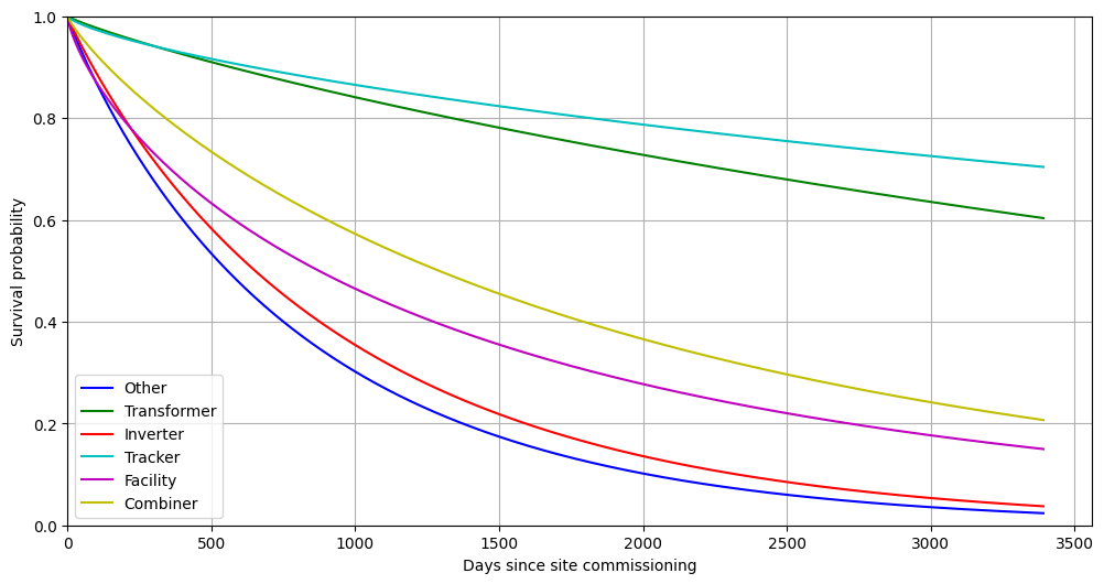
Weibull distribution fitting
The Weibull distribution describes a family of probability distributions parametrized by a shape parameter and a scale parameter. It is frequently used to model the probability of failure by fitting its parameters to observed data. As a parametric method, it is less flexible than the nonparametric Kaplan-Meier estimation but is simpler and potentially easier to interpret.
The models.survival.fit_survival_function in the pvops.timeseries module implements the Weibull fitting when method=weibull' is used, shown below.
[7]:
col_dict = {'group_by': 'Asset', 'time_to_fail': 'days_until_failure', 'was_observed': 'was_observed'}
weibull_results = timeseries.models.survival.fit_survival_function(censored_om_df, col_dict, method='weibull')
And we can plot the Weibull results as well:
[8]:
plt.figure(figsize=(12,6))
assets = om_df['Asset'].unique()
colors = list(plt.cm.colors.BASE_COLORS.values())[:len(assets)]
days = range(censored_om_df['days_until_failure'].max())

for asset, color in zip(assets, colors):
    fitted_weibull = weibull_results[asset]['distribution']
    weibull_probs = fitted_weibull.sf(days)
    plt.plot(days, weibull_probs, color=color, label=asset)

plt.legend();
plt.grid();
plt.xlim(0,None);
plt.ylim(0,1);
plt.xlabel('Days since site commissioning')
plt.ylabel('Survival probability');
We can also extract the coefficients and format them into a table for analysis:
[10]:
parameters = [list(series.values())[:-1] for series in weibull_results.values()]
param_df = pd.DataFrame(parameters, index=weibull_results.keys(), columns=['shape', 'scale'])
param_df
[10]:
| shape | scale | |
|---|---|---|
| Other | 0.932064 | 823.962180 |
| Transformer | 0.875983 | 7396.679666 |
| Inverter | 0.943692 | 961.246107 |
| Tracker | 0.724652 | 14380.096078 |
| Facility | 0.742765 | 1430.950715 |
| Combiner | 0.850317 | 1986.362160 |
We can see that all asset types have shape parameters < 1, indicating the rates of failure decreases over time for all asset types. Inverters see the slowest reduction in failure rate, while trackers have the fastest.