IV Simulator Tutorial
A python class which simulates PV faults in IV curves.
Step 1: Start off by instantiating the object.
[1]:
from pvops.iv import simulator

sim = simulator.Simulator()
Step 2: Definition of Faults
Two methods exist to define a fault:
Use a pre-existing definition (defined by authors) by calling
add_preset_conditions.Manually define a fault by calling
add_manual_condition.
Preset definition of faults
[2]:
heavy_shading = {'identifier':'heavy_shade',
                   'E': 400,
                   'Tc': 20}
light_shading = {'identifier':'light_shade',
                    'E': 800}
sim.add_preset_conditions('landscape', heavy_shading, rows_aff = 2)
sim.add_preset_conditions('portrait', heavy_shading, cols_aff = 2)
sim.add_preset_conditions('pole', heavy_shading, light_shading = light_shading, width = 2, pos = None)

sim.print_info()
Condition list: (Cell definitions)
        [pristine]: 1 definition(s)
        [heavy_shade]: 1 definition(s)
        [light_shade]: 1 definition(s)

Modcell types: (Cell mappings on module)
        [pristine]: 1 definition(s)
        [landscape_2rows]: 1 definition(s)
        [portrait_2cols]: 1 definition(s)
        [pole_2width]: 1 definition(s)

String definitions (Series of modcells)
        No instances.
Manual definition of faults
To define a fault manually, you must provide two specifications:
Mapping of cells onto a module, which we call a
modcell.Definition of cell conditions, stored in
condition_dict.
[3]:
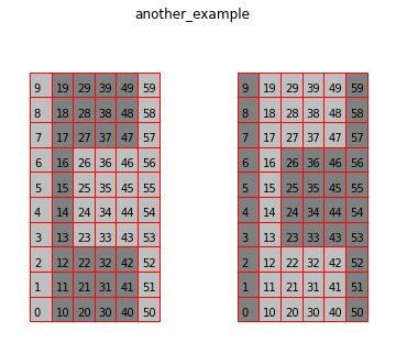
modcells = { 'another_example':  [[0,0,0,0,0,0,0,0,0,0,  # Using 2D list (aka, multiple conditions as input)
                                    1,1,1,1,1,1,1,1,1,1,
                                    1,1,1,0,0,0,0,1,1,1,
                                    1,1,1,0,0,0,0,1,1,1,
                                    1,1,1,0,0,0,0,1,1,1,
                                    0,0,0,0,0,0,0,0,0,0],

                                  [1,1,1,1,1,1,1,1,1,1,
                                    0,0,0,0,0,0,0,0,0,0,
                                    0,0,0,1,1,1,1,0,0,0,
                                    0,0,0,1,1,1,1,0,0,0,
                                    0,0,0,1,1,1,1,0,0,0,
                                    1,1,1,1,1,1,1,1,1,1]]
            }
condition_dict = {0: {},
                  1: {'identifier': 'heavy_shade',
                      'E': 405,
                     }
                 }
sim.add_manual_conditions(modcells, condition_dict)

sim.print_info()
Condition list: (Cell definitions)
        [pristine]: 1 definition(s)
        [heavy_shade]: 2 definition(s)
        [light_shade]: 1 definition(s)

Modcell types: (Cell mappings on module)
        [pristine]: 1 definition(s)
        [landscape_2rows]: 1 definition(s)
        [portrait_2cols]: 1 definition(s)
        [pole_2width]: 1 definition(s)
        [another_example]: 2 definition(s)

String definitions (Series of modcells)
        No instances.
Step 3: Generate many samples via latin hypercube sampling
Pass in dictionaries which describe a distribution.
    {PARAMETER: {'mean': MEAN_VAL,
                 'std': STDEV_VAL,
                 'low': LOW_VAL,
                 'upp': UPP_VAL
                }
    }

PARAMETER: parameter defined in condition_dict
If all values are provided, a truncated gaussian distribution is used
If low and upp not specified, then a gaussian distribution is used
[4]:
N = 10
dicts = {'E': {'mean': 400,
               'std': 500,
               'low': 200,
               'upp': 600},

         'Tc':{'mean': 30,
               'std': 10}}


sim.generate_many_samples('heavy_shade', N, distributions = dicts)

dicts = {'E': {'mean': 800,
               'std': 500,
               'low': 600,
               'upp': 1000}}

sim.generate_many_samples('light_shade', N, distributions = dicts)

sim.print_info()
Condition list: (Cell definitions)
        [pristine]: 1 definition(s)
        [heavy_shade]: 12 definition(s)
        [light_shade]: 11 definition(s)

Modcell types: (Cell mappings on module)
        [pristine]: 1 definition(s)
        [landscape_2rows]: 1 definition(s)
        [portrait_2cols]: 1 definition(s)
        [pole_2width]: 1 definition(s)
        [another_example]: 2 definition(s)

String definitions (Series of modcells)
        No instances.
Step 4: Define a string as an assimilation of modcells
Define a dictionary with keys as the string name and values as a list of module names.
{STRING_IDENTIFIER: LIST_OF_MODCELL_NAMES}
Use sim.modcells.keys() to get list of modules defined thusfar, or look at modcell types list in function call sim.print_info()
[3]:
sim.modcells.keys()
[3]:
dict_keys(['pristine', 'landscape_2rows', 'portrait_2cols', 'pole_2width'])
[5]:
sim.build_strings({'pole_bottom_mods': ['pristine', 'pristine', 'pristine', 'pristine', 'pristine', 'pristine',
                                        'pole_2width', 'pole_2width', 'pole_2width', 'pole_2width', 'pole_2width', 'pole_2width'],
                   'portrait_2cols_3bottom_mods': ['pristine', 'pristine', 'pristine', 'pristine', 'pristine', 'pristine',
                                                   'pristine', 'pristine', 'pristine', 'portrait_2cols', 'portrait_2cols', 'portrait_2cols']})
Step 5: Simulate!
sim.simulate() simulates all cells, substrings, modules, and strings defined in steps 2 - 4
[6]:
import time
start_t = time.time()
sim.simulate()
print(f'\nSimulations completed after {round(time.time()-start_t,2)} seconds')

sim.print_info()
Simulating cells:   0%|                                                                          | 0/3 [00:00<?, ?it/s]c:\users\mwhopwo\appdata\local\programs\python\python36\lib\site-packages\scipy\optimize\zeros.py:463: RuntimeWarning: some failed to converge after 100 iterations
  warnings.warn(msg, RuntimeWarning)
Simulating cells: 100%|██████████████████████████████████████████████████████████████████| 3/3 [00:01<00:00,  2.93it/s]
Adding up simulations: 100%|█████████████████████████████████████████████████████████████| 2/2 [00:09<00:00,  4.66s/it]
Adding up other definitions: 100%|███████████████████████████████████████████████████████| 5/5 [00:01<00:00,  3.62it/s]
Simulations completed after 11.74 seconds
Condition list: (Cell definitions)
        [pristine]: 1 definition(s)
        [heavy_shade]: 12 definition(s)
        [light_shade]: 11 definition(s)

Modcell types: (Cell mappings on module)
        [pristine]: 1 definition(s)
        [landscape_2rows]: 1 definition(s)
        [portrait_2cols]: 1 definition(s)
        [pole_2width]: 1 definition(s)
        [another_example]: 2 definition(s)

String definitions (Series of modcells)
        [pole_bottom_mods]: 132 definition(s)
        [portrait_2cols_3bottom_mods]: 12 definition(s)
Step 6: Visualization suite
Plot distribution of cell-condition parameter definitions defined in steps 2 and 3
1a) TODO: The truncated gaussians should show cutoff at tails
Plot module-level IV curves
Plot string-level IV curves
[7]:
sim.visualize()


Step 6 cont’d: Visualize cell IV curves and settings
visualize_cell_level_traces(cell_identifier, cutoff = True, table = True)
Automatically turns off table if the cell_identifier’s number of definitions > 20
[8]:
sim.visualize_cell_level_traces('heavy_shade', cutoff = True, table = True)
sim.visualize_cell_level_traces('light_shade', cutoff = True, table = True)
[8]:
array([<matplotlib.axes._subplots.AxesSubplot object at 0x000001A4685F5D68>,
       <matplotlib.axes._subplots.AxesSubplot object at 0x000001A4686300B8>],
      dtype=object)


Step 6 cont’d: Visualize modcells
[9]:
for mod_identifier in sim.modcells.keys():
    sim.visualize_module_configurations(mod_identifier, title = mod_identifier)