Timeseries Tutorial

This notebook demonstrates the use of timeseries module capabilities to process data for analysis and build expected energy models.

[20]:

import numpy as np
import pandas as pd
import matplotlib.pyplot as plt
import os
import warnings
warnings.filterwarnings("ignore")

[21]:

from pvops.timeseries import preprocess
from pvops.timeseries.models import linear, iec
from pvops.text2time import utils as t2t_utils, preprocess as t2t_preprocess

[22]:

example_prodpath = os.path.join('example_data', 'example_prod_with_covariates.csv')

Load in data

[23]:

prod_data = pd.read_csv(example_prodpath, on_bad_lines='skip', engine='python')

Production data is loaded in with the columns: - date: a time stamp - randid: site ID - generated_kW: generated energy - expected_kW: expected energy - irrad_poa_Wm2: irradiance - temp_amb_C: ambient temperature - wind_speed_ms: wind speed - temp_mod_C: module temperature

[24]:

prod_data.head()

[24]:

	date	randid	generated_kW	expected_kW	irrad_poa_Wm2	temp_amb_C	wind_speed_ms	temp_mod_C
0	2018-04-01 07:00:00	R15	0.475	0.527845	0.02775	16.570	4.2065	14.1270
1	2018-04-01 08:00:00	R15	1332.547	1685.979445	87.91450	16.998	4.1065	15.8610
2	2018-04-01 09:00:00	R15	6616.573	7343.981135	367.90350	20.168	4.5095	24.5745
3	2018-04-01 10:00:00	R15	8847.800	10429.876422	508.28700	21.987	4.9785	30.7740
4	2018-04-01 11:00:00	R15	11607.389	12981.228814	618.79450	23.417	4.6410	35.8695

[25]:

metadata = pd.DataFrame()
metadata['randid'] = ['R15', 'R10']
metadata['dcsize'] = [20000, 20000]
metadata.head()

[25]:

	randid	dcsize
0	R15	20000
1	R10	20000

Column dictionaries

Create production and metadata column dictionary with format {pvops variable: user-specific column names}. This establishes a connection between the user’s data columns and the pvops library.

[26]:

prod_col_dict = {'siteid': 'randid',
                 'timestamp': 'date',
                 'powerprod': 'generated_kW',
                 'irradiance':'irrad_poa_Wm2',
                 'temperature':'temp_amb_C', # Optional parameter, used by one of the modeling structures
                 'baseline': 'IEC_pstep', #user's name choice for new column (baseline expected energy defined by user or calculated based on IEC)
                 'dcsize': 'dcsize', #user's name choice for new column (System DC-size, extracted from meta-data)
                 'compared': 'Compared',#user's name choice for new column
                 'energy_pstep': 'Energy_pstep', #user's name choice for new column
                 'capacity_normalized_power': 'capacity_normalized_power', #user's name choice for new column
}

metad_col_dict = {'siteid': 'randid',
                  'dcsize': 'dcsize'}

Data Formatting

Use the prod_date_convert function to convert date information to python datetime objects and use prod_nadate_process to handle data entries with no date information - here we use pnadrop=True to drop such entries.

[27]:

prod_data_converted = t2t_preprocess.prod_date_convert(prod_data, prod_col_dict)
prod_data_datena_d, _ = t2t_preprocess.prod_nadate_process(prod_data_converted, prod_col_dict, pnadrop=True)

Assign production data index to timestamp data, using column dictionary to translate to user columns.

[28]:

prod_data_datena_d.index = prod_data_datena_d[prod_col_dict['timestamp']]

min(prod_data_datena_d.index), max(prod_data_datena_d.index)

[28]:

(Timestamp('2018-04-01 07:00:00'), Timestamp('2019-03-31 18:00:00'))

[29]:

prod_data_datena_d

[29]:

	date	randid	generated_kW	expected_kW	irrad_poa_Wm2	temp_amb_C	wind_speed_ms	temp_mod_C
date
2018-04-01 07:00:00	2018-04-01 07:00:00	R15	0.475	0.527845	0.02775	16.570000	4.2065	14.127000
2018-04-01 08:00:00	2018-04-01 08:00:00	R15	1332.547	1685.979445	87.91450	16.998000	4.1065	15.861000
2018-04-01 09:00:00	2018-04-01 09:00:00	R15	6616.573	7343.981135	367.90350	20.168000	4.5095	24.574500
2018-04-01 10:00:00	2018-04-01 10:00:00	R15	8847.800	10429.876422	508.28700	21.987000	4.9785	30.774000
2018-04-01 11:00:00	2018-04-01 11:00:00	R15	11607.389	12981.228814	618.79450	23.417000	4.6410	35.869500
...	...	...	...	...	...	...	...	...
2019-03-31 14:00:00	2019-03-31 14:00:00	R10	19616.000	20179.797303	967.10350	-4.129722	5.9935	35.860694
2019-03-31 15:00:00	2019-03-31 15:00:00	R10	19552.000	20149.254116	983.94500	-4.214444	5.1770	38.549306
2019-03-31 16:00:00	2019-03-31 16:00:00	R10	19520.000	20192.672439	1011.77950	-3.943611	4.2430	42.848889
2019-03-31 17:00:00	2019-03-31 17:00:00	R10	17968.000	19141.761319	895.76800	-4.124167	3.1885	42.321806
2019-03-31 18:00:00	2019-03-31 18:00:00	R10	11616.000	12501.159607	649.48700	-4.663056	2.2540	38.596944

8755 rows × 8 columns

Data Preprocessing

Preprocess data with prod_inverter_clipping_filter using the threshold model. This adds a mask column to the dataframe where True indicates a row to be removed by the filter.

[30]:

masked_prod_data = preprocess.prod_inverter_clipping_filter(prod_data_datena_d, prod_col_dict, metadata, metad_col_dict, 'threshold', freq=60)

filtered_prod_data = masked_prod_data[masked_prod_data['mask'] == False]

print(f"Detected and removed {sum(masked_prod_data['mask'])} rows with inverter clipping.")

Detected and removed 24 rows with inverter clipping.

Normalize the power by capacity

[31]:

for site in metadata[metad_col_dict['siteid']].unique():
    site_metad_mask = metadata[metad_col_dict['siteid']] == site
    site_prod_mask = filtered_prod_data[prod_col_dict['siteid']] == site
    dcsize = metadata.loc[site_metad_mask, metad_col_dict['dcsize']].values[0]
    filtered_prod_data.loc[site_prod_mask, [prod_col_dict['capacity_normalized_power']]] = filtered_prod_data.loc[site_prod_mask, prod_col_dict['powerprod']] / dcsize

Visualize the power signal versus covariates for one site with normalized values.

[32]:

temp = filtered_prod_data[filtered_prod_data['randid'] == 'R10']
for xcol in ['irrad_poa_Wm2', 'temp_amb_C', 'wind_speed_ms']:
    plt.scatter(temp[xcol], temp[prod_col_dict['capacity_normalized_power']])
    plt.title(xcol)
    plt.grid()
    plt.show()

../../_images/pages_tutorials_tutorial_timeseries_22_0.png

../../_images/pages_tutorials_tutorial_timeseries_22_1.png

../../_images/pages_tutorials_tutorial_timeseries_22_2.png

Dynamic linear modeling

We train a linear model using site data (irradiance, temperature, and windspeed)

[33]:

model_prod_data = filtered_prod_data.dropna(subset=['irrad_poa_Wm2', 'temp_amb_C', 'wind_speed_ms']+[prod_col_dict['powerprod']])
# Make sure to only pass data for one site! If sites are very similar, you can consider providing both sites.
model, train_df, test_df = linear.modeller(prod_col_dict,
                                           kernel_type='polynomial',
                                           #time_weighted='month',
                                           X_parameters=['irrad_poa_Wm2', 'temp_amb_C'],#, 'wind_speed_ms'],
                                           Y_parameter='generated_kW',
                                           prod_df=model_prod_data,
                                           test_split=0.05,
                                           degree=3,
                                           verbose=1)

train {1, 2, 3, 4, 5, 6, 7, 8, 9, 10, 11, 12}
Design matrix shape: (8293, 108)
test {2, 3}
Design matrix shape: (437, 108)

Begin training.
[OLS] Mean squared error: 679448.77
[OLS] Coefficient of determination: 0.99
[OLS] 108 coefficient trained.
[RANSAC] Mean squared error: 812510.79
[RANSAC] Coefficient of determination: 0.98

Begin testing.
[OLS] Mean squared error: 7982573.16
[OLS] Coefficient of determination: 0.85
[OLS] 108 coefficient trained.
[RANSAC] Mean squared error: 81461712.61
[RANSAC] Coefficient of determination: -0.55

Define a plotting function

[34]:

from sklearn.metrics import mean_squared_error, r2_score

def plot(model, prod_col_dict, data_split='test', npts=50):

    def print_info(real,pred,name):
        mse = mean_squared_error(real, pred)
        r2 = r2_score(real, pred)
        print(f'[{name}] Mean squared error: %.2f'
                % mse)
        print(f'[{name}] Coefficient of determination: %.2f'
                % r2)

    fig,(ax) = plt.subplots(figsize=(14,8))

    if data_split == 'test':
        df = test_df
    elif data_split == 'train':
        df = train_df

    measured = model.estimators['OLS'][f'{data_split}_y'][:npts]

    ax2 = ax.twinx()
    ax2.plot(model.estimators['OLS'][f'{data_split}_index'][:npts], df[prod_col_dict['irradiance']].values[:npts], 'k', label='irradiance')

    ax.plot(model.estimators['OLS'][f'{data_split}_index'][:npts], df['expected_kW'].values[:npts], label='partner_expected')
    print_info(measured, df['expected_kW'].values[:npts], 'partner_expected')

    ax.plot(model.estimators['OLS'][f'{data_split}_index'][:npts], measured, label='measured')
    for name, info in model.estimators.items():
        predicted = model.estimators[name][f'{data_split}_prediction'][:npts]
        ax.plot(model.estimators[name][f'{data_split}_index'][:npts], predicted, label=name)
        print_info(measured, predicted, name)

    ax2.set_ylabel("Irradiance (W/m2)")
    ax.set_ylabel("Power (W)")
    ax.set_xlabel('Time')
    handles, labels = [(a+b) for a, b in zip(ax.get_legend_handles_labels(), ax2.get_legend_handles_labels())]
    ax.legend(handles, labels, loc='best')
    plt.show()

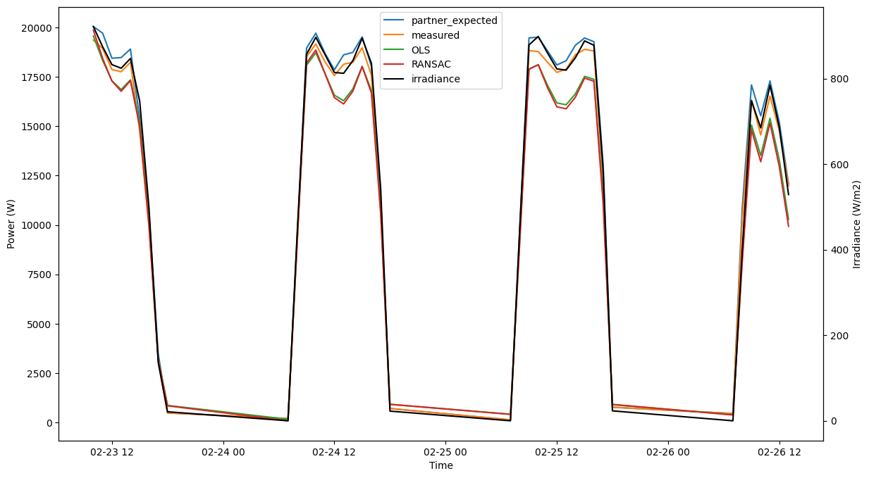
Observe performance

[35]:

plot(model, prod_col_dict, data_split='train', npts=40)

[partner_expected] Mean squared error: 2883252.79
[partner_expected] Coefficient of determination: 0.93
[OLS] Mean squared error: 225151.82
[OLS] Coefficient of determination: 0.99
[RANSAC] Mean squared error: 253701.63
[RANSAC] Coefficient of determination: 0.99

../../_images/pages_tutorials_tutorial_timeseries_28_1.png

[36]:

plot(model, prod_col_dict, data_split='test', npts=40)

[partner_expected] Mean squared error: 273446.60
[partner_expected] Coefficient of determination: 0.99
[OLS] Mean squared error: 1037605.79
[OLS] Coefficient of determination: 0.98
[RANSAC] Mean squared error: 1300872.49
[RANSAC] Coefficient of determination: 0.97

../../_images/pages_tutorials_tutorial_timeseries_29_1.png